Mobile robot autonomy · Python · from scratch

navstack
a 2D autonomy stack, built from the math up

A differential-drive robot is dropped into a world it has never seen. It maps the space from LiDAR, works out where it is despite odometry that drifts without bound, explores until nothing is left unknown, plans a route, drives it, and replans when someone puts a box in the corridor. Every algorithm underneath is implemented by hand.

numpy · pygame · matplotlib no ROS no nav2 no gmapping / cartographer no off-the-shelf planners or filters mypy --strict clean

What it does

Seven subsystems, one integration state machine, and a hard rule about ground truth.

0.036 m
MCL tracking error over a two-minute patrol
0.36 m
Raw wheel odometry on the same run, still growing
100%
Of reachable area mapped, exploring autonomously (best of 3 seeds — see limitations)
100%
A* success across 100 verified-solvable pairs
The full stack, unedited. Grey is mapped free space, white is mapped obstacle, and the dark background is still unknown. Pink dots are the particle cloud, the blue line is the current plan. Nothing here reads the simulator's true state.

The rule that shapes everything

Ground truth lives in the simulator and nowhere else.

Mapping, localization, planning and control may only ever consume what a real robot would have: a LidarScan and a drifting OdomReading. Ground-truth maps are produced only by explicitly-named constructors that stamp a known_map provenance flag, so a demo running on a handed-to-it map cannot report itself as having mapped anything. The true pose appears in the live view only beneath a line that says diagnostics only.

That constraint is what makes the rest of the project mean anything. It is also why the odometry has to genuinely drift — if dead reckoning were good enough, the particle filter would be decoration.
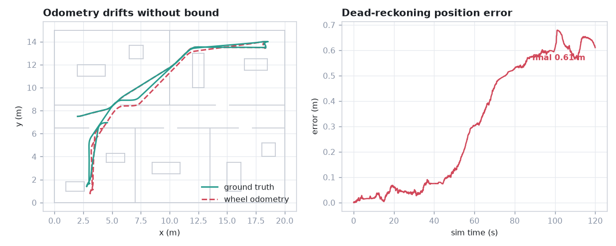
Left: ground-truth trajectory versus wheel odometry diverging over a patrol. Right: dead-reckoning error growing to 0.61 m.
Odometry drifts without bound: each step's heading error rotates every subsequent displacement, so position error compounds rather than averaging out.

Localization

A particle filter, and the two ways it fails.

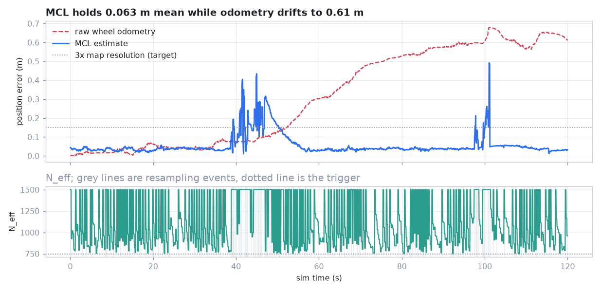
A Kalman filter represents belief as a single Gaussian, so it cannot express “I am in one of four identical corridors” — the mean of two hypotheses is a pose inside a wall. A particle filter can, and pays for it with sampling failure modes instead. Both are demonstrated here rather than described.

MCL error holding near 0.06 m while odometry drifts to 0.61 m, with N_eff and resampling events below.
Top: MCL against raw odometry. Bottom: effective sample size, with the resampling trigger dotted — resampling only when N_eff degrades is what stops a healthy filter throwing away its own diversity.
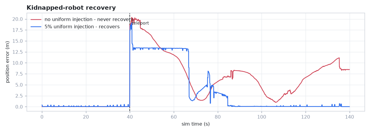
Kidnapped-robot experiment: without uniform injection the error stays at 8.8 m; with 5% injection it returns to 0.07 m.
The kidnapped-robot experiment: 28.8 m of permanent error becomes 0.04 m. Resampling can only pick particles it already has, so after a teleport the filter is confidently and permanently wrong — and injection alone does not save it, because a uniformly-wrong cloud has high N_eff and never triggers a resample. Augmented MCL watches the level of sensor agreement instead of its spread, and fires when it collapses.
Tempering — an exponent on the summed log-likelihood — rescues global localization from particle deprivation, because 30 LiDAR beams on one flat wall are not 30 independent observations. Tracking is near-indifferent to it. An earlier version of this page claimed tempering harmed tracking, citing a real 3.87 m measurement; the damage was actually the motion model mishandling reverse motion during recovery. A plausible story fitted to a real number is still the wrong story.

Planning

A* wins at 2D. The interesting question is why you would ever use RRT.

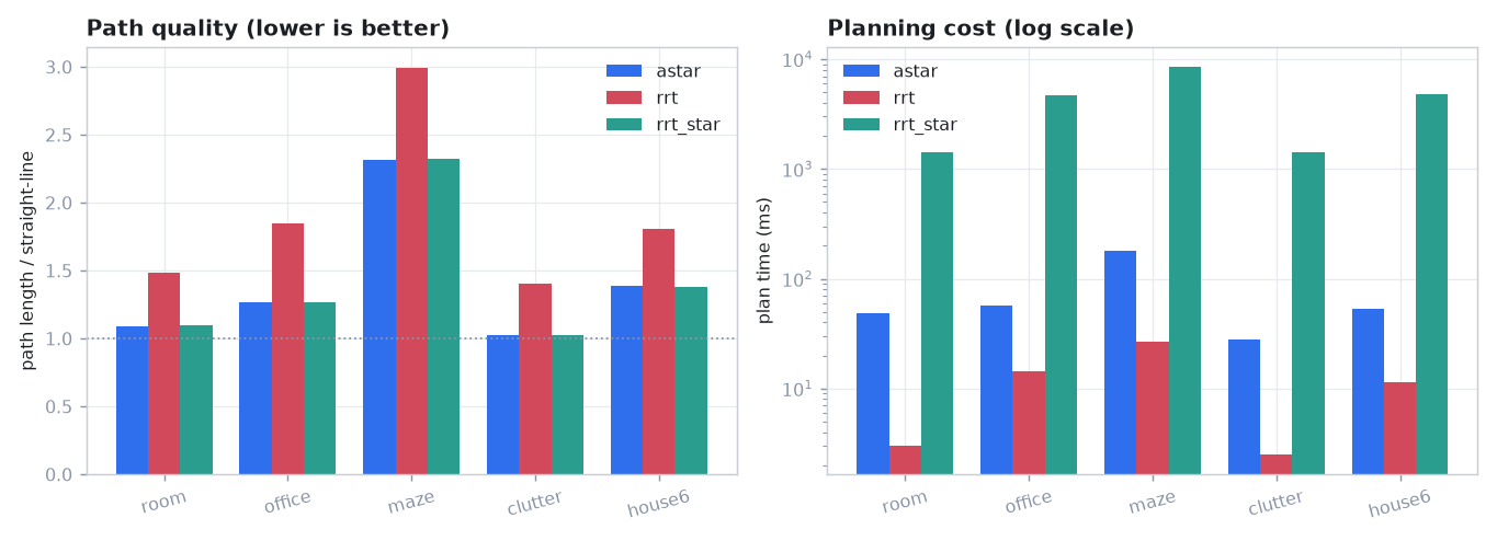
Twenty randomized start/goal pairs per world. Every pair is verified connected by a flood fill before it is used, so a reported failure is a real planner failure and not an impossible instance — reporting success rates against unsolvable problems is the most common way planner benchmarks lie. Every returned path is re-checked for collisions before it counts.

WorldPlannerSuccesslen / lower boundWorkPlan time
officeA*100%1.277046 expansions42 ms
officeRRT100%1.85543 nodes11 ms
officeRRT*100%1.275000 nodes1429 ms
mazeA*100%2.3112402 expansions185 ms
mazeRRT100%2.99859 nodes28 ms
mazeRRT*100%2.325000 nodes2444 ms
clutterA*100%1.022754 expansions18 ms
clutterRRT100%1.41107 nodes2 ms
clutterRRT*100%1.035000 nodes1044 ms
Bar charts comparing path length ratio and planning time for A*, RRT and RRT* across five worlds.
RRT plans 4–20× faster but 30–60 % longer. RRT* recovers A*-quality paths at 20–50× A*'s cost, because it never terminates early by design.

So at 2D, A* simply wins. The reason to have RRT at all is dimensional: A* costs O(cells) and cells grow exponentially with degrees of freedom, so the ranking in that table inverts long before you reach a 6-DOF arm, where a grid is not implementable at all.

Replanning

A failed plan is a result, not a retry condition.

A box appears in the corridor. The robot sees it on LiDAR, the map updates, the current path stops being clear, and the executive replans around it. If the corridor is genuinely sealed it reports UNREACHABLE and stops — because replanning every control step against a closed corridor burns CPU, keeps commanding motion into the obstacle, and never tells anyone. An early version did exactly that: 2721 replans and 2644 collisions in one run.

Obstacle dropped mid-drive. Detour found in two replans, zero collisions.

There is also a RECOVERING state, which exists because pure pursuit only drives forwards. An obstacle appearing close ahead can leave the robot pressed against it inside the planner's inflation margin, facing the wrong way — a pose from which every valid plan begins with a manoeuvre the tracker cannot execute.

Bugs worth reading about

Found by tests and benchmarks. Each one has a regression test.

  1. The textbook exact-integration formula annihilates its own answer. R·[sin(θ+φ) − sin θ] with R = v/ω loses about three decimal digits by φ = 1e-7, and by φ = 1e-8 the cosine difference underflows to exactly zero — the lateral displacement is not approximated, it is destroyed. Rewriting product-to-sum removes the cancellation and needs no small-angle branch at all.
  2. A vectorized DDA is not Bresenham. Rounding disagrees with the error accumulator on roughly a quarter of integer lines. The accumulator turns out to have a closed form, ⌊(2k·d + n − 1)/2n⌋, whose − 1 is the tie-break. Verified byte-identical on 5000 random lines.
  3. Path smoothing vetoed the wrong thing. Checking that a relaxed waypoint sits in free space says nothing about the leg joining it to its neighbour, which can sweep straight through a wall corner.
  4. Sampled collision checks disagree with themselves. Splitting a segment changes which points get sampled, so a verified path fails after being densified without moving. Fixed with exact grid traversal — whose boundary crossings must be recomputed rather than accumulated, since the accumulated form drifts within a hundred cells.
  5. The planner and its own replan trigger disagreed. A* snapped a blocked start out of the inflation margin; the clearance check did not. Every freshly planned path was therefore declared blocked the instant it was returned.
  6. The odometry motion model cannot represent reverse motion. A backward step gives rot1 ≈ π, so the model believes the robot spun round and drove off, while the noise terms — which scale with rot1² — explode. The executive reverses on purpose during recovery, so every recovery destroyed the filter: 0.09 m → 11.2 m. It was first misdiagnosed as a tuning problem, and the wrong conclusion reached the docs before the real cause was found.
  7. Zeroing odometry on collision is wrong twice over. It discards rotation that physically happened, and it hides wheel slip — one of the largest real sources of odometry error. A real encoder counts turns of the wheel, not displacement of the robot.

Run it

Clone to live demo in under ten minutes.

# the whole stack: unknown world, mapped from LiDAR, localized with MCL,
# explored autonomously, then navigated to a goal — on estimated state only
python3.11 -m venv .venv && .venv/bin/pip install -e ".[dev]"
.venv/bin/python demos/demo.py --world maps/house6.json --goal storage

# a maze it has never seen, and an ablation with the filter switched off
.venv/bin/python demos/demo.py --world maps/unseen_maze.txt
.venv/bin/python demos/demo.py --world maps/house6.json --known-pose

# reproduce every number and figure on this page
.venv/bin/python -m pytest
.venv/bin/python tools/benchmark.py
.venv/bin/python tools/plots.py

Source is not published yet — the repository link goes here.

Limitations

Stated, not hidden.

  • The full-stack demo succeeds on one seed in three. The bar was three out of three on an unseen maze. Measured over an 800 s budget: seed 0 maps 100 % and reaches its goal, seed 2 reaches 92.5 % and runs out of time, seed 1 stalls at 40 %. Every subsystem meets its own criterion; the integration is what is seed-dependent, and the fix is scan matching and loop closure rather than more tuning.
  • Global localization fails in a highly self-similar maze. The corridors are genuinely ambiguous, and a weighted-mean estimate is meaningless across multiple modes. Reporting the largest cluster would be the honest fix; it is not implemented.
  • SLAM is not properly closed. The full demo maps from the filter's own estimate against a map it is simultaneously building. There is no loop closure and no pose-graph optimisation, so a long enough run will drift.
  • Exploration is greedy. No tour planning, so it can leave a pocket behind and cross the whole map for it later.
  • RRT* has no anytime termination. It always runs to max_nodes.
  • Pure pursuit only. DWA was scoped as a stretch goal and dropped, so there is no local reactive layer.

What I would do next

In order.

  • EKF-SLAM on the same worlds, same sensors and metrics, so the Gaussian-versus-multi-modal trade-off becomes a measurement instead of an assertion.
  • Pose-graph loop closure — the actual fix for the drift limitation.
  • DWA as a local layer, benchmarked on reaction time to a suddenly appearing obstacle versus full replanning.
  • 3D and 6-DOF, where the benchmark's conclusion inverts and RRT* stops being a curiosity.
  • A ROS 2 port of the interfaces; the module boundaries were drawn with node boundaries in mind.